数值分析作业 - 插值
数值分析Problem 1

Lagrange 插值:
Newton 插值:
插值的结果是相同的.
Problem 2

Problem 3
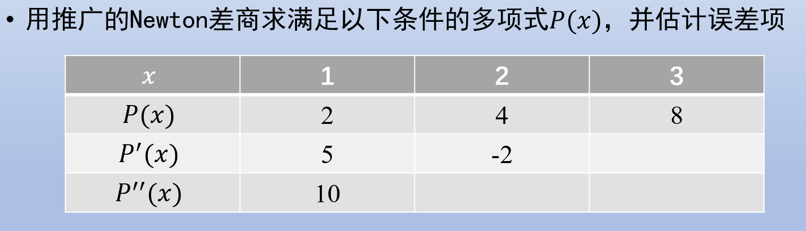
Problem 4
下面的 Mathematica 程序给定插值点和函数值, 计算 Newton 差商矩阵的第一行
1 | newtonCoeffcient[xi_?ListQ, fi_?ListQ] := Module[{a, n, c}, ( |
先使用 Mathematica 内置的 InterpolatingPolynomial 计算插值多项式
1 | xi = {0, \[Pi]/6, \[Pi]/3, \[Pi]/4, \[Pi]/2}; |
再使用 Newton 法计算
1 | cNewton = newtonCoeffcient[xi, fi] // Simplify; |
1 | pNewton = newtonValue[xi, cNewton, x] // Expand; |
得到的结果与内置函数完全一致.
将给定点直接代入插值函数求近似值, 在
1 | x = N[{1, 2, 3, 4, 14, 1000}]; |
利用三角函数的周期性
1 | pSin[x_] := Piecewise[{ |
得到的结果是合理的
绝对误差
1 | Map[pSin, x] - Sin[x] // TeXForm |
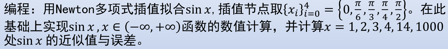
可以注意到绝对误差均在小数点后三位.
1 | Plot[pSin[x] - Sin[x], {x, 0, \[Pi]/2}] |
Problem 5

定义一些辅助的变量和函数
1 | uniformSample[a_, b_, n_] := Range[a, b, (b - a)/(n - 1)]; |
取
1 | Clear[x]; |
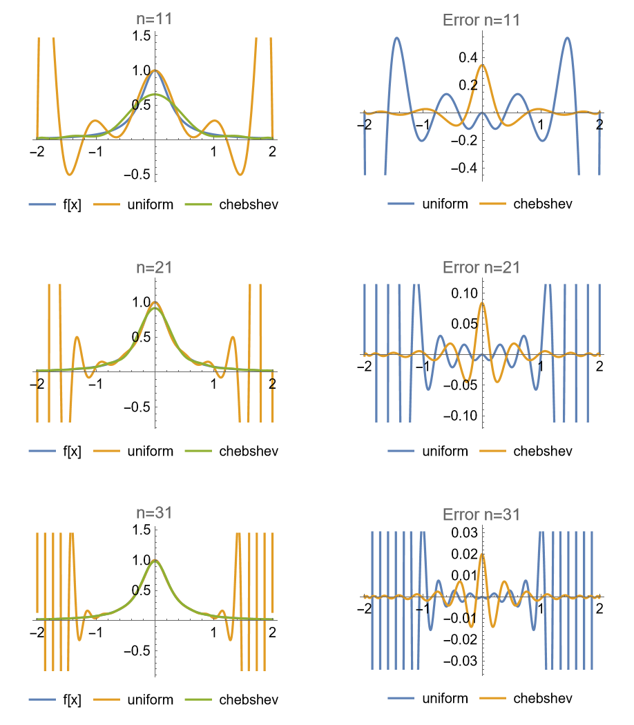
注意到, 在中间的
Problem 6

实现三次自然样条插值
1 | splineCoefficient[xi_?ListQ, fi_?ListQ] := |
并绘制图形
1 | GraphicsGrid[ParallelMap[Module[{xi, data}, |
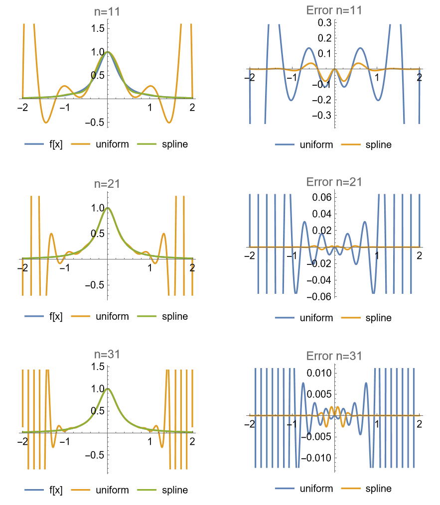
可以注意到样条法不会发生端点附近剧烈震荡的情况, 误差也要小于高次插值, 但是参数量较大.
许可协议
本文采用 署名-相同方式共享 4.0 国际 许可协议,转载请注明出处。
分享文章


