微分方程数值解作业 3
微分方程Problem 1
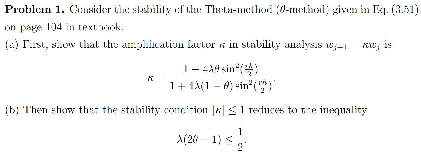
Question (a)
Assume (3.30)
and substitute it into (3.51)
With setting
Collecting terms with
Use the identity
Then use
Finally, we have
which contains the desired
Question (b)
The stability condition is
Breakdown the absolute value, we have
Since
which holds irrespective of the value of
Problem 2

Question (a)
The stencil is shown below.
Limits on
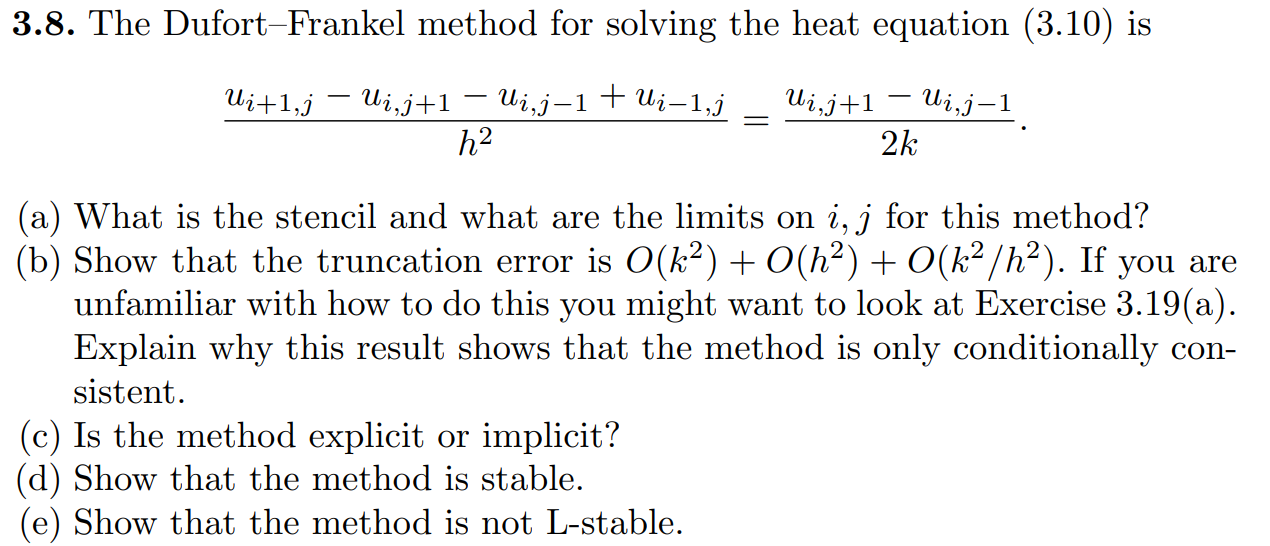
Question (b)
FDE for the Dufort-Frankel scheme is
Extract
Use
This is of order
Question (c)
The method is explicit.
Question (d)
Use
Extract
Substitute
Assume
which yields the following 2nd order equation
The roots of this equation are
For the method to be stable, we need
For complex roots where
and
Note that
Question (e)
From
This indicates that though
Problem 3

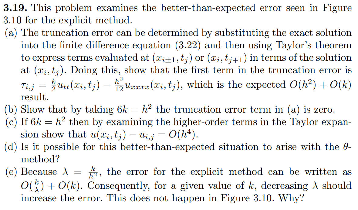
Question (a)
From equation (3.22)
we can replace terms with Taylor expansion at
Cancel duplicated terms, we have
where
Question (b) (c)
Taking
When applied to the heat equation
we have
assuming
Therefore, we can see that the
Question (d)
Apply Taylor expansion to
And extract
It is possible but tedious to show that
Question (e)
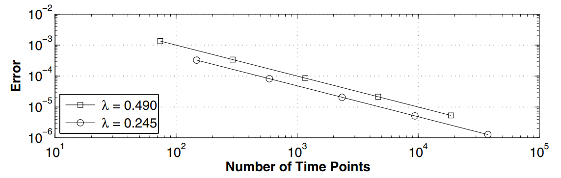
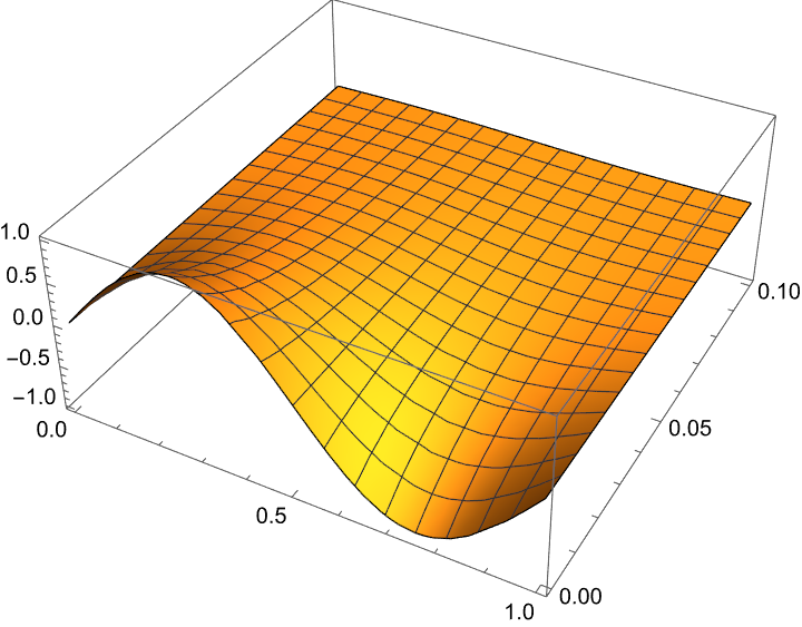
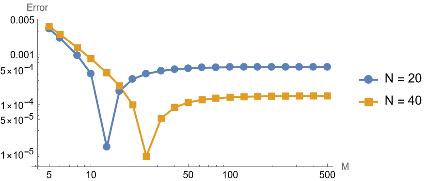
In the above sub-figure,
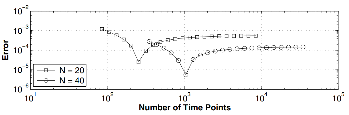
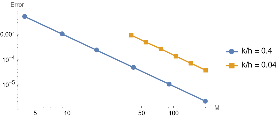
This sub-figure has fixed
Problem 4
Question (a)
1 | makeAMatrix[n_, \[Lambda]_] := |
Check the code with the following test case
1 | f = Function[{x, t}, 0]; |
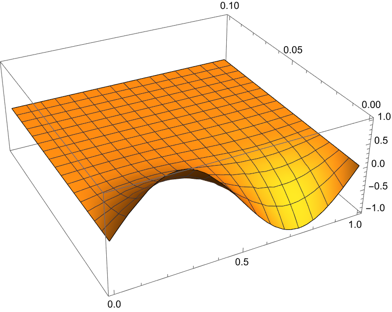
Find the analytical solution
1 | exactsol = |
Then define functions to make error plot
1 | makeFigure315[f_, g_, n_, ms_, td_, tp_, it_, exact_] := Module[{sols}, |
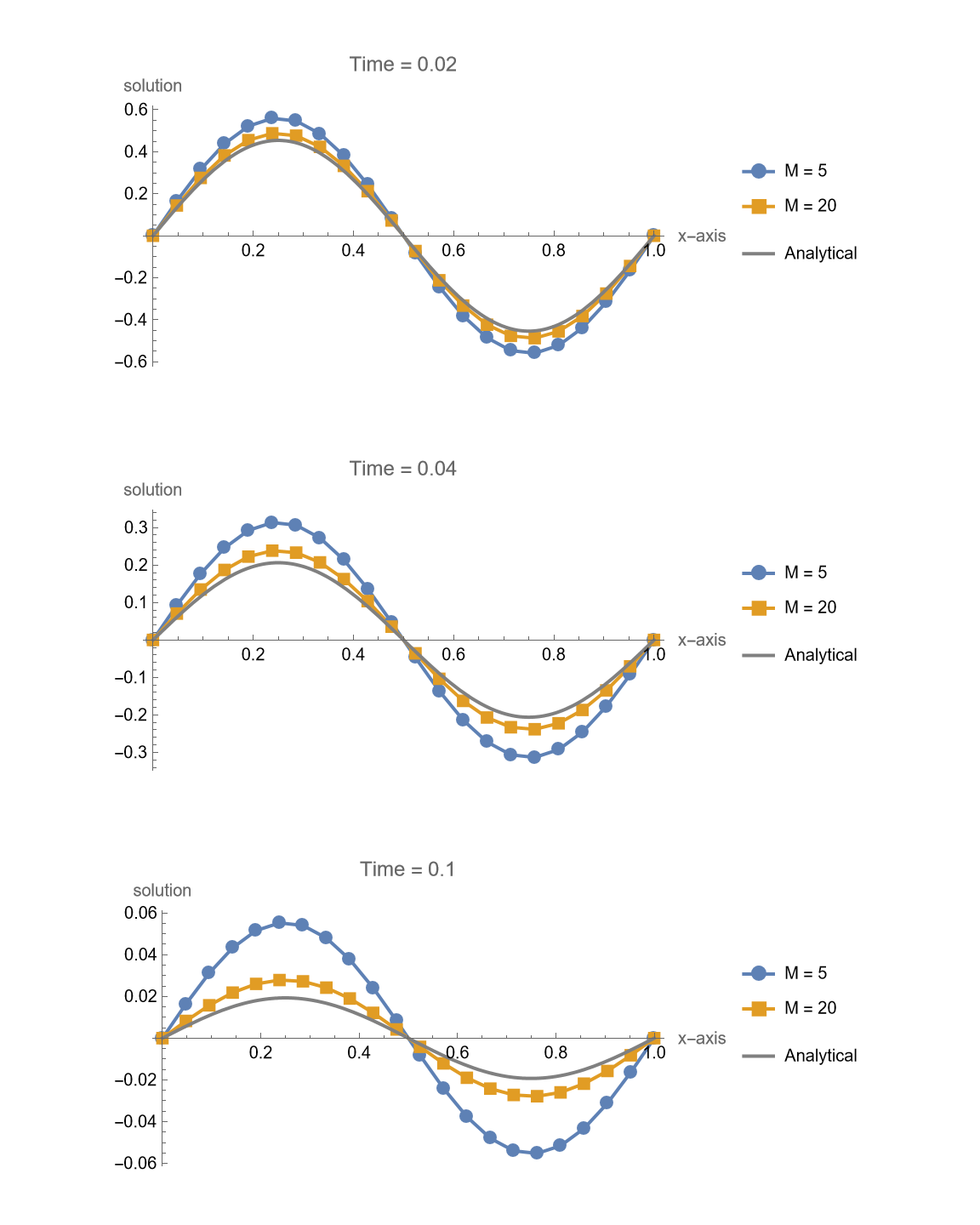
Explicit Method
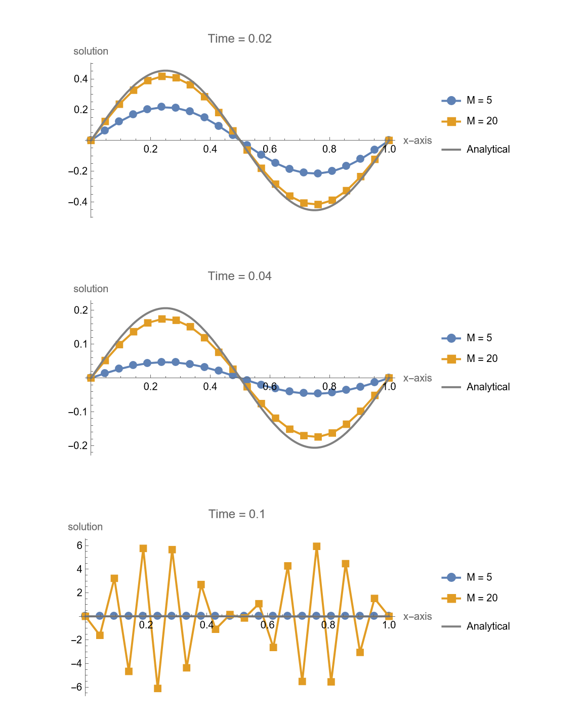
1 | makeFigure315[f, g, 20, {5, 20}, 0.1, {0.02, 0.04, 0.1}, explicitIt, exactsol] |
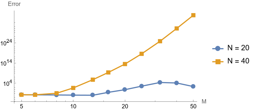
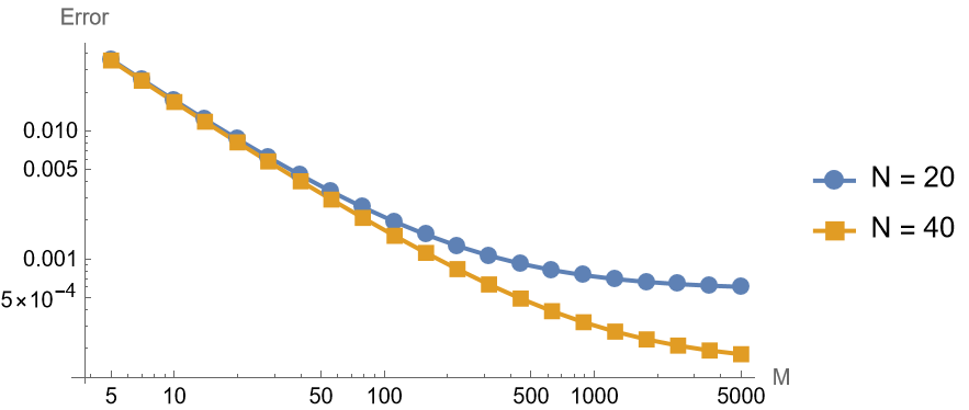
1 | makeFigure316FixedN[f, g, {20, 40}, 10, 50, 0.1, explicitIt, exactsol] |
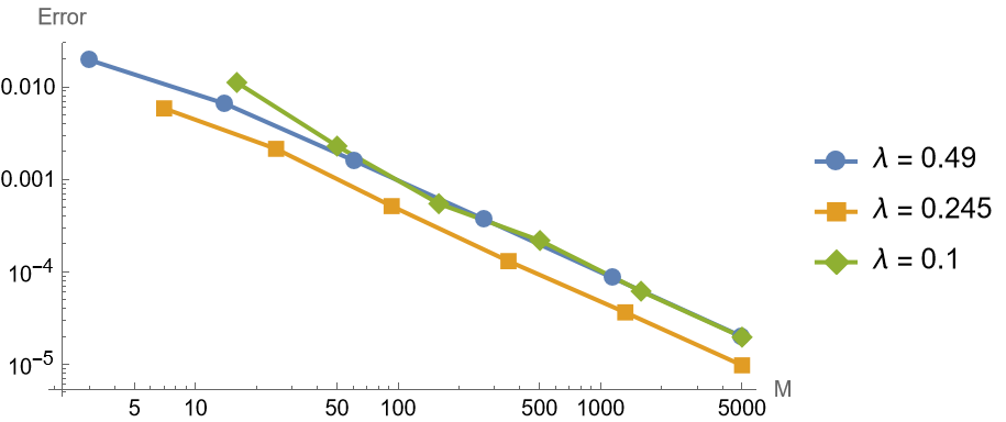
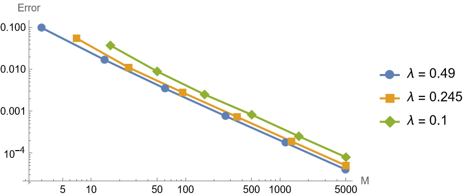
1 | makeFigure316FixedLambda[f, g, {0.490, 0.245, |
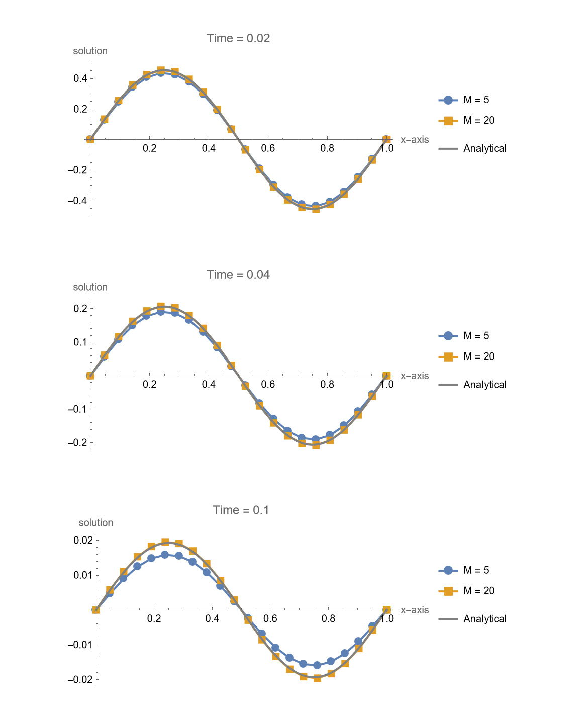
Implicit Method
1 | makeFigure315[f, g, 20, {5, 20}, 0.1, {0.02, 0.04, 0.1}, implicitIt, exactsol] |
1 | makeFigure316FixedN[f, g, {20, |
1 | makeFigure316FixedLambda[f, g, {0.490, 0.245, |
Crank-Nicolson Method
1 | makeFigure315[f, g, 20, {5, 20}, 0.1, {0.02, 0.04, 0.1}, crankNicolsonIt, exactsol] |
1 | makeFigure316FixedN[f, g, {20, |
1 | makeFigure316FixedKH[f, g, {0.4, |
Question (b)
First find the analytical solution
1 | exactsol = |
Calculating the infinite sum is not feasible, we simply limit the sum to
1 | exactfun = |
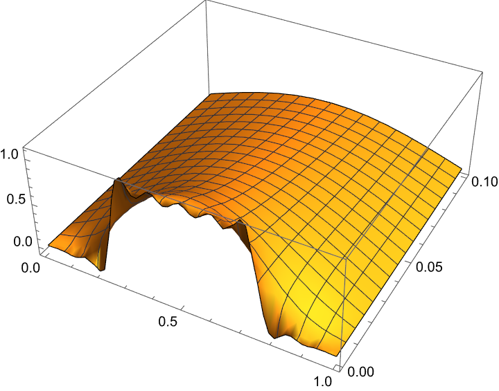
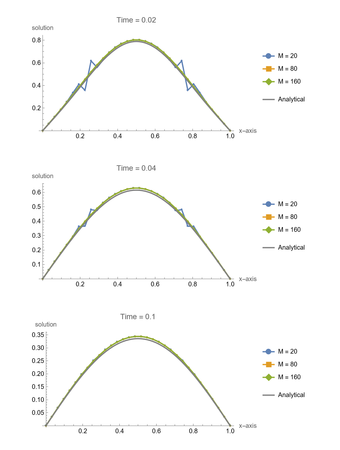
Loss in high frequency is observed where
1 | makeFigure317[f_, g_, n_, ms_, td_, tp_, it_, exact_] := Module[{sols}, |
Implicit Method
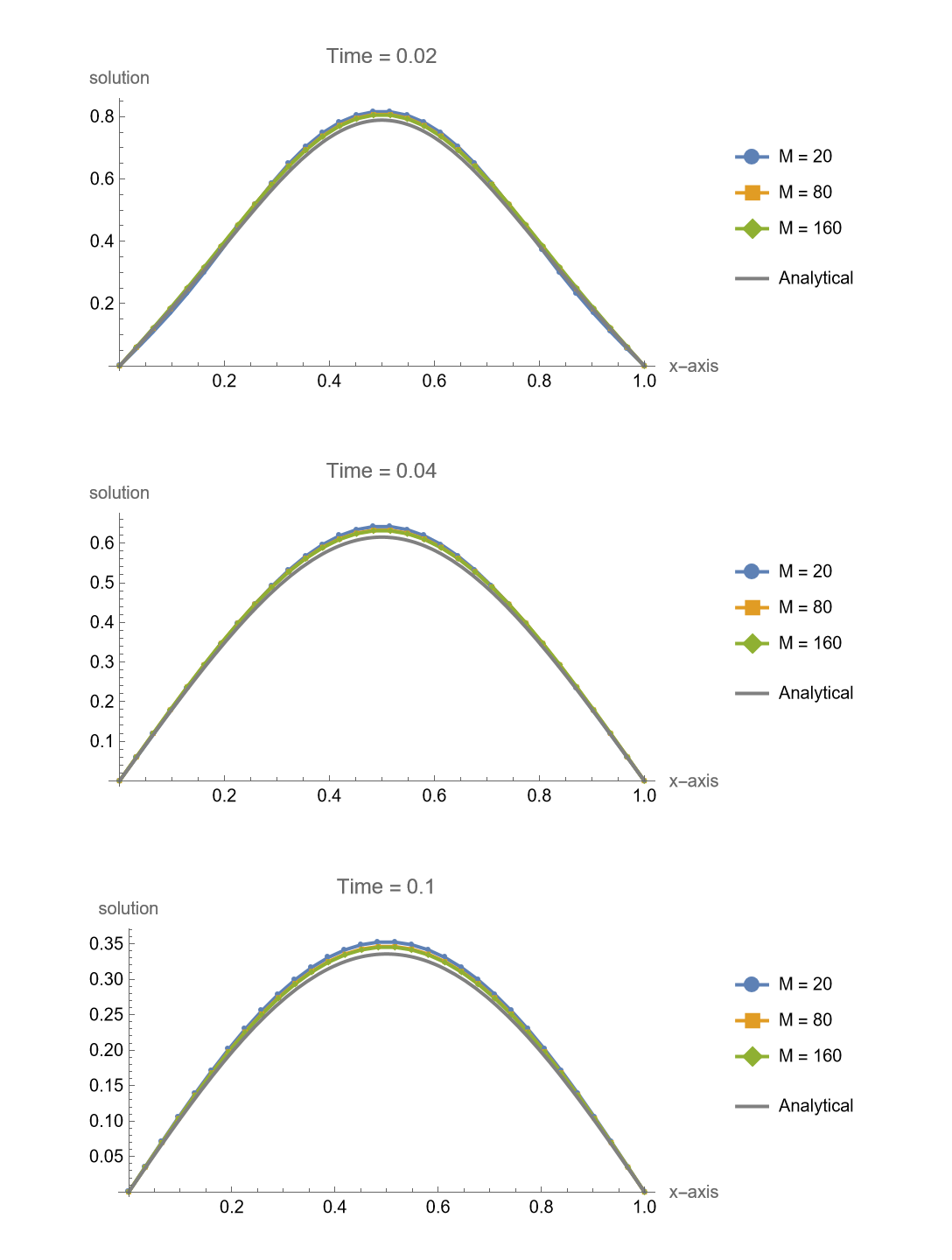
1 | makeFigure317[f, g, 30, {20, 80, 160}, 0.1, {0.02, 0.04, |
Crank-Nicolson Method
1 | makeFigure317[f, g, 30, {20, 80, 160}, 0.1, {0.02, 0.04, |
For Crank-Nicolson method, the amplification factor
Though
本文采用 署名-相同方式共享 4.0 国际 许可协议,转载请注明出处。


