微分方程数值解作业 5

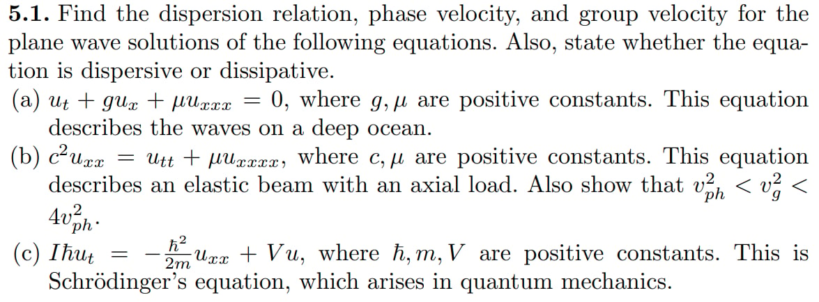
Problem 1

Question (a)

With the plane wave solution

we have

That simplifies to

which holds for all if and only if

and this is the dispersion relation. The phase velocity

The group velocity

The equation is dispersive since depends on . The equation is nondissipative since requires to be zero.

Question (b)

With the plane wave solution, we have

That simplifies to

Therefore the dispersion relation is

Since are all real, is real. The phase velocity

The phase velocity

The group velocity

It can be shown that

Also,

which is true since is positive.

The equation is dispersive since depends on . It is also disspative because in , is not necessarily real.

Question (c)

With the plane wave solution, we have

which simplifies to

The dispersion relation is

The phase velocity

The group velocity

The equation is dispersive since depends on . It is also nondissipative since is zero.

Problem 2

Question (a)

Question (b)

From (5.31) we have

With the initial condition in we have

That is

All desired can be solved by the tridiagonal matrix equation

And then compute using , and so on.

Question (c)

The method satisfies CFL condition, since the system described by requires depends on all of , so the numerical domain of dependence is the entire domain. As shown in previous chapters, an unnecessarily large domain of dependence can lead to less accurate results. Using other approximations in space can not lift the need to solve the tridiagonal matrix equation.

Question (d)

From (5.31) we have

With the initial condition in we have

Therefore can be determined explicitly by

The stencil for is , which is a 3-point stencil.

The CFL condition is the same as in the textbook.

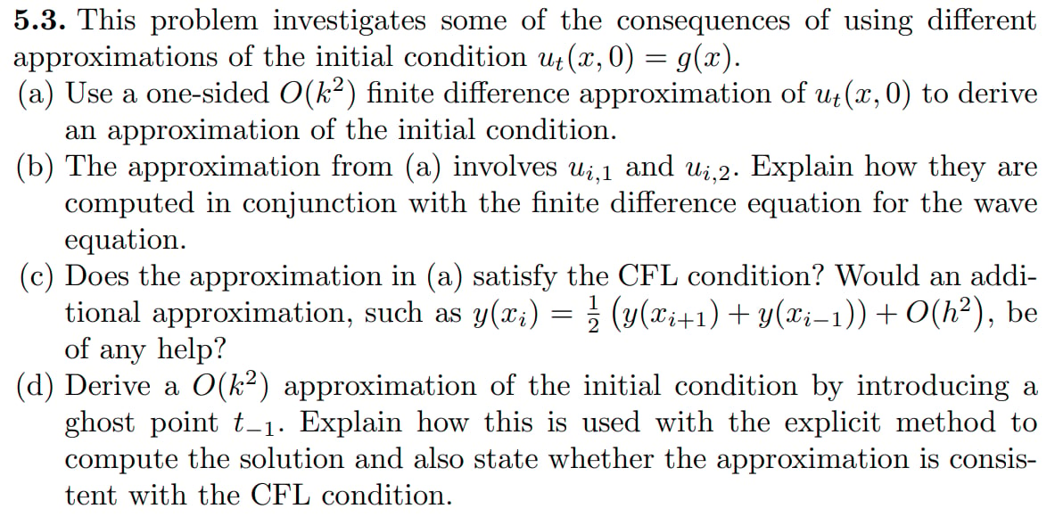
Problem 3

Question (a)

1. Use a uniform grid where and
2. Evaluate the difference equation at
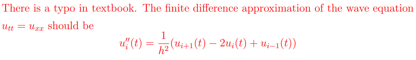
3. Using centered differences to approximate the derivatives we have This can be rearranged to where is the truncation error.
4. Drop the error term to get the finite difference approximation for and . The first boundary condition in (5.2) can be approximated by The second boundary condition in (5.3) can be handled by introducing ghost points at , described in . With we can calculate for

The stencil for this method is

and

at the first time step The numerical domain of dependence consists of the points

The damped wave equation can be considered as a wave equation combined with a diffusion equation. The wave equation has a finite domain of dependence, while the diffusion equation propagates information instantaneously. Therefore the domain of dependence of the damped wave equation is the entire domain. Thus explicit methods can never satisfy the CFL condition.

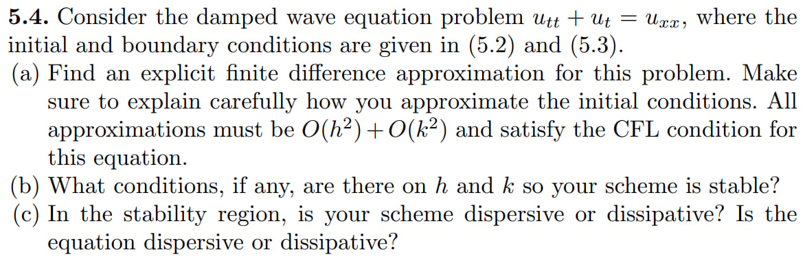
Question (b)

Assuming

we can substitute this into to obtain

The amplification factor is

From some numerical experiments we can find that the magnitude of the amplification factor is less than 1 for all positive . The method is always stable.

Question (c)

First we investigate the dispersion relation of the damped wave equation

Substituting the plane wave solution, we have

and the dispersion relation is

The phase velocity is

and depends on . Therefore the damped wave equation is dispersive. is not zero, so the equation is dissipative.

Then we investigate the dispersion relation of the finite difference method. The numerical plane wave solution is

Substituting this into we have

It will be difficult to solve , but it can be shown that always depends on and has a non-zero imaginary part. Therefore the finite difference method is dispersive and dissipative, matching the properties of the damped wave equation.

Problem 4

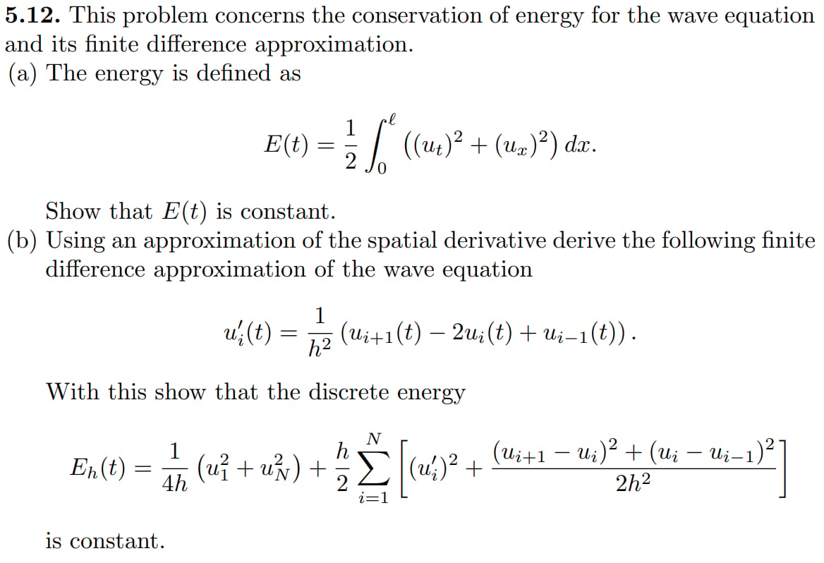
Question (a)

With the wave equation

we have . Therefore is a constant.

Question (b)

The discrete energy is

and the approximation of the wave equation is